DevRel – What is that?

Almost a year ago, I heard the term DevRel for the first time when Sara Safavi, from Planet, gave a talk at CodeOp and used that word to describe her new role. I knew Sara as a developer, like myself, so I was curious to learn what this role entailed and understand how it could attract someone with a strong technical background.

It turns out that DevRel – Developer Relations – is as close as you can be to the developer world, without actually writing code. All these things that I used to do in my spare time, like participating in hackathons, writing blog posts, participating in conversations on Twitter, speaking at events, are now the core part of my job. I did them, because they are fun, and also because I believe that ultimately, writing code has an impact in society, and in order to run that last mile we need to get out of our compilers and reach out to the world. Technology is like a piece of art – it only fulfills its mission when it leaves the artist’s basement and it reaches the museums, or at least the living room of someone who appreciates it.

I am happy to say that I am now the DevRel at the Open Geospatial Consortium. In a way, it is a bit ironic that I ended up taking this role in an organization that does not actually produce software as its main outcome. But in a way OGC is the ultimate software facilitator, by producing the standards that will be used by developers to build their interoperable, geospatial aware, products and services. If you are reading this and you are not a geogeek, you may think of W3C as a somehow similar organization: it produces the HTML specification, which is not itself a software, but how could we build all these frontend applications using React, Vue and so many other frameworks, without using HTML? It is that important. Now you may be thinking, “so tell me an OGC standard that I use, or at least know”, and, again, if you are not a geogeek, maybe you won’t know any of the standards I will mention. Even if you use, or have used at some point location data. And this is part of the reason why I am at OGC.

Location data is increasingly part of the mainstream. We all carry devices in our pockets that produce geo referenced data with an accuracy that was undreamed ten years ago. Getting hold of these data opens a world of possibilities for data scientists and data engineers, but in order for all these applications to be able to understand each other we need sound, well articulated standards in place. My main goal as DevRel at OGC will be to bring the OGC standards closer to the developer community, by making them easier to use, and by making sure that they are actually used. And maybe, just maybe, I will also get to write some code along the way.

Interactive Maps within React.js

Recently, I have been teaching a Full-stack development bootcamp at CodeOp (great experience!).

When the students reached project phase, I was very pleased to see a lot of interest in using maps. And that is easy to understand, right? geospatial information is associated to most activities these days (e.g.: travel, home exchange, volunteering), and interactive maps are the backbone of any application which uses geospatial information.

This made me think of a nice way of introducing the students to interactive mapping. I realized that most of them want to do one thing: read an address and display it on the map, which also requires the use of a geocoder. In order to demonstrate how to put all these things together within a React application, which is the framework they are using, I created a small demo on GitHub. This was also an opportunity to practice and improve my front end skills! 🙂

Following a good tradition of GitHub, I started by forking an existing project, which I thought was similar to what I wanted to achieve. Although the project is extremely cool, I realized that I wanted to move in quite a different direction, so I ended up diverging a lot from the original code base.

To implement the map, I used my favourite library for interactive maps, Leaflet. This library is actually packaged as a React component, so it is really easy to incorporate it into an application.

Of course, maps only understand coordinates, and most of the time people have nominal locations such as street names, cities, or even postcodes. This was also the case with my students. Translating strings with addresses to a pair of coordinates is not a trivial task, so the best thing is to leave it up to the experts. I used the Open Cage geocoder, an API to convert coordinates to and from places. Why? It has a much more generous free tier than the Google Maps API, and it is open-source. And although it is built on top of OSM Nominatum, it contains several improvements.

The good news are OpenCage also has a package for JavaScript and Node, and it is really easy to use. This is the piece of code, to retrieve the coordinates from a given string:

    // Adds marker to map and flies to it with an animation
    addLocation =() =>{
      opencage
        .geocode({ q: this.state.input, key: OCD_API_KEY})
        .then(data => {
          // Found at least one result
          if (data.results.length > 0){
              console.log("Found: " + data.results[0].formatted);
              const latlng = data.results[0].geometry;
              const {markers} = this.state
              markers.push(latlng)
              console.log(latlng);
              this.setState({markers})
              let mapInst =  this.refs.map.leafletElement;
              mapInst.flyTo(latlng, 12);
          } else alert("No results found!!");

        })
        .catch(error => {
          console.log('error', error.message);
        });


    }

In order to do this, you need to sign up for a free API key first, and store it within a secrets file (.env).

The application allows the user to type any address, and it will fly to it with an animation, adding a marker on the map.

You can check out the final result at https://leaflet-react.herokuapp.com/

 

 

FindMeACoin: a Platform to Support Offline Trading of Cryptocurrencies

Trading crypto currency offline¹, in person, is the quickest way of acquiring/selling crypto coins. It is also the only way of not exposing any identity information.

This post presents a platform for finding buyers/sellers for crypto currencies in a certain geographic location. Registered users can find other users on a map, and get in touch with them to arrange a meeting.

The collected information about the users is kept at the bare minimum.

The platform only puts users in touch. It does not participate or interfere in the trading process, and thus it does not take any liability for what may happen. However, if the transaction is successful it does collect a fee, based on a smart contract.

The platform uses a gamification approach, with the use of avatars, associated to reputation. It aims to be kept simple and user friendly.

At this stage we are looking forward to collecting expressions of interest, and feedback in general. If you want to be the first to try FindMeACoin, please register now!

FindMeACoin is a platform which enables users to trade cryptocurrencies, in a private, reliable, easy and fun way.

Let’s make transactions private again!

1In this context, trading currencies “offline” means trading currencies in person, converting from cash to a cryptocurrency, or vice versa.

 

Spatial Data Mining

Social media streams may generate massive clouds of geolocated points, but how can we extract useful information from these, sometimes huge, datasets? I think machine learning and GIS can be helpful here.

My PechaKucha talk at DataBeers : “Visualizing Geolocated Tweets: a Spatial Data Mining Approach”.

Driving Spatial Analysis Beyond the Limits of Traditional Storage

My presentation on the “Conference on Advanced Spatial Modelling and Analysis” consisted in some thoughts regarding Big Spatial Data, and how to handle them in terms of modern technologies.

It was great to see such a motivated crowd from all generations, and to get to know the research developed by CEG, in topics such as Agent Based Modelling and Neural Networks. It was also great to talk again to Arnaud Banos, from the Complex System Institute of Paris Ile-de-France (ISC-PIF).

Importing Large Spatial Datasets into PostGIS

Is PostgreSQL/PostGIS suitable for Big Data? This is a question I have been asking myself for a while, and I now have the opportunity to test it with a PostgreSQL instance from Amazon Web Services (AWS); after all, if such a service cannot deal with “Big Data”, who can?
I have a dataset with Tweets in the city of Barcelona, over a time period. The entire dataset amounts to about 3 million points (82 MB), and I have some subsets: a smaller collection of about 2 million points (55 MB) and 300 000 points (8.2. MB).

We can argue whether this dataset is, or not, Big Data; but IMHO, a table with more than 1 million records starts to get “heavy” for any relational database. Now before doing any computations of spatial algorithms (e.g.: convex hull, point in polygon), the very first step is to actually load this dataset into the database. And this is where I started to struggle.

QGIS has a plugin called SPIT, that allows to import a Shapefile into PostGIS. Unfortunately it seems to be extremely slow any of the three files that I mentioned above (including the smaller one).

Switching to the command line, where I have more control knowledge about the processes that are running, I tried shp2pgsql, a tool for importing Shapefiles that comes with the PostGIS installation.

On Linux it is possible to convert and import the Shapefile in one go, redirecting the output with pipe:

shp2pgsql -s <SRID> -c -D -I <path to shapefile> <schema>.<table> | \
psql -d <databasename> -h <hostname> -U <username>

Since this command was really slow (unresponsive?) I decided to do it in two steps, to see where it was hanging:

• Create an sql file with the insert statements.
• Load this sql file into the database.

Unsurprisingly, the SQL file with the statements was generated quite quickly, and the processing effort was being spent on the insert queries. This situation was verified with the three Shapefiles, even when I inserted a spatial index (Gist). After thinking a bit, I came to the conclusion that the spatial index should be created within the “CREATE TABLE” statement, so it should actually speed up the queries a bit (but I did not confirm this guess).

My next attempt, was to use ogr2ogr, the GDAL tool to convert between vector formats.

ogr2ogr -f "PostgreSQL" PG:"host=host user=user dbname=db password=pass" data.shp

I have to say that I read some suggestion to prefer shp2pgsql over this tool, and in fact it was quite slow as well (at this point I was only testing the smallest of the Shapefiles).

My conclusion up to this moment, is that it is quite expensive in terms of time (and processor) to import a large dataset into a PostGIS. Some ideas that could be explored:

• Upgrade the PostGIS server (would scale vertically make any difference?).
• Upload the data into the Amazon server and run the import tool from there. I am not sure whether it is possible to do that, but it seems like a good improvement to do this operation locally, and using the power of the Amazon Server, rather than my desktop computer.
• Split the Shapefile into chunks of data. I am not entirely sure how to do this, and any suggestions would be welcome.

Next steps: once I manage to import a large Shapefile into my PostGIS instance, I will post some feedback about the computation of spatial operations.

Update: Apparently I underestimated the fact that I am importing data over a network connection, with a limited latency. The best thing would be to make the import locally, an option that I unfortunately don’t have, since the Amazon RDS does not give me SSH access (it is a service, not a machine!). I decided to switch to a new approach: import a plain csv file into a database table, using the /copy command, and that was actually really fast (a few seconds).

psql database -U user -h host.eu-west-1.rds.amazonaws.com -c "\copy newt_table from 'data.csv' with DELIMITER ','"

Of course, I then had to run a query populate the point geometry from the float (x,y) values, and create an update a spatial index (for a matter efficiency it is recommended that indexes are created after, and not during the import!).

UPDATE new_table SET geom = ST_SetSRID(ST_MakePoint(lon,lat),4326);

CREATE INDEX [indexname] ON [tablename] USING GIST ( [geometryfield] );

VACUUM ANALYZE [table_name] [column_name];

That was still considerably fast (although not as much as the csv import!), and my guess is: it is because I are now running queries on the remote machine (and not uploading data via an internet connection).

Following some very usefull on Stack Overflow, I decided to retry my previous approaches, tuning the configuration parameters.

First I tried the OGR command line tool, but this time with the config flag “PG_USE_COPY YES”, to force dumping of the data:

ogr2ogr -progress -f PostgreSQL PG:"dbname='database' user='user' host='host.eu-west-1.rds.amazonaws.com' port='5432' data.shp --config PG_USE_COPY YES -nlt POINT -nln import_ogr

Although speed has improved massively, it still took me 1:03:00 to run this query.

Then I tried the shp2pgsql tool, with the “-D” flag, which also forces the dump of data:

shp2pgsql -D -s 4326 data.shp import_shp2pgsql | psql

This was remarkably fast: 00:01:04

Comparing the two imports, we can see that shp2pgsql did not create any index (which we already commented is a costly operation), while ogr2ogr created a gist index on the spatial field. The extra step of creating an index, has to be added to the shp2pgsql import, but as we have seen before, that operation is not a problem since we are then operating on the server.

I conclude this review, stating that shp2pgsql has a great performance in the task of  loading a Big Data spatial table into a remote PostGIS server (e.g.: Amazon RDS). It is recommended that the “-D” flag is passed to the tool, and that no indexes are created during this operation.

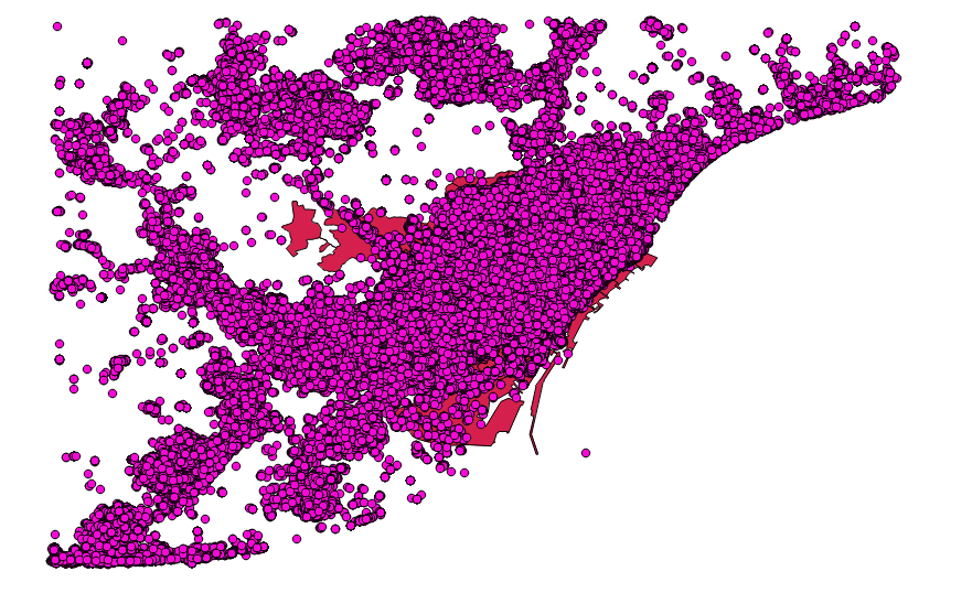
Bellow we can see the PostGIS geometry of the imported table, with more than 3 million points:

Clustering Geospatial Data

Recently I have been looking into different algorithms for the clustering geospatial data. The problem of finding “similar” regions in space, is a very interesting one, since this type of classification enables a whole range of applications (e.g.: urban development, transport planning, etc).
When we are working with “Big Data”, as the one resultant from streaming of crowd sourced date (for instance), the amount of information makes it difficult to visually detect things; this is often where artificial intelligence can “give us an hand”.

DBSCAN is a density-based clustering algorithm, that can find an, a priori unknown, number of clusters with an arbitrary shape. It starts with a certain “idea” of what a cluster is, based on a density as defined by its parameters: epsilon and minpts. This “idea” is also the main weakness of DBSCAN, as the global parameters, don’t allow to capture different densities in the dataset, if that is the case; and often, in geographical datasets, it is.

In the example above, we can see that a different value of epsilon, and therefore a different threshold of density, yields very different results. With the larger epsilon we detect clusters around all the AOI, but the centre comes up as a single cluster. With the smaller epsilon, we have more detail in the centre, but we “loose” the less dense clusters in the outskirts. In a way, DBSCAN corresponds to looking at the data with “semi closed” eyes, and this is why its results make so much sense to the user.

OPTICS is considered a generalization of DBSCAN, tackling exactly these difficulty in configuring the parameters, by becoming almost parameterless. Instead of using an epsilon to limit the search for neighbours, OPTICS considers a range of epsilons, up to a maximum, that could be a radius that includes the entire AOI (although for practical purposes, you don’t really want to do that, because it increases the complexity of the algorithm). OPTICS is essentially an ordering of the database, such as points that are spatially closest become neighbours in the ordering. The output of optics is a graphic plotting this ordering, and a special distance that is stored for each point, representing the density that needs to be accepted for a cluster in order to have both points belong to the same cluster; this is called a dendrogram.

source: wikipedia

OPTICS does not produce a strict partitioning of the data, but this can be done using algorithms, that try to identify the “peaks” and “valleys” in the graphic, or by selecting a range of x and a threshold of y (xi). Generally speaking these algorithms produce a hierarchical clustering, which is more difficult to interpret than the “flat” partitioning produced by DBSCAN. Conceptually, this OPTICS output would correspond to many “runs” of DBSCAN.

There are implementations of DBSCAN and OPTICS in the WEKA and ELKI libraries. WEKA’s implementation of DBSCAN has been thoroughly referred as slow, when compared to ELKI’s implementation. This benchmarking illustrates well the difference between the two. Although some improvements were added in the latest versions of WEKA, this difference was confirmed by invoking the two algorithms in some test cases. OPTICS implementation in WEKA does not produce a classification. In ELKI’s library, the OPTICS algorithm is separated from the classification algorithm, following ELKI’s modular philosophy; ELKI’s OPTICSxi produces a clustering classification, using a partitioning algorithm selected (or implemented) by the user.

DBSCAN is very sensitive to its two parameters, which are quite hard to setup. Also, the parameters “influence” each other in the result. They are hard to setup because they depend largely on the particular phenomena we are studying, and which type of clusters we want to detect. If we want to identify “meaningful” things, we need to have a pretty good idea of what we are looking for. If a good domain knowledge is strongly advised, it is also advised to inspect the results of the clustering algorithm, by plotting them in a map. For all these reasons, I think that DBSCAN is very good as a exploratory tool, for producing meaningful and scientific analysis about a dataset, but I don’t see it as very “realistic” to implement it as part of a “service” that automatically analyses any dataset, “on demand”.

OPTICS seems a bit more “obscure” to me. The algorithm is more sophisticated than DBSCAN, in the sense that it has a more “flexible” idea of a cluster, but it produces a more complex result, which is more difficult for the user to interpret. OPTCIS itself does not produce any classification, so the quality of the cluster “results”, actually heavily depend on the algorithm that we choose to perform the partition.

In a way, I don’t see OPTICS as a “replacement” for DBSCAN, but as a complement. It allows us to detect some “patterns” that are not “visible” to DBSCAN, but the lack of global parameters does not allow us to capture the “global” structure of the dataset.