Mapping the IVAucher

As a reaction to the record high of fuel prices, the Portuguese government has updated the IVAucher program, to allow each citizen to recover 10 cents per each liter of fuel spent, up to a maximum of 5 EUR/month. This blog post is not going to discuss whether this is good way of spending the public budget, or if it is going to make a real impact in the lives of the people that manage to subscribe to this program. Instead, I want to focus on data.

Once you subscribe to the program as a consumer, you just need to fill the tank in one of the gas stations that subscribed the program, as businesses. The IVAucher website publishes a list of subscribed stations, which seems to be updated, from time to time. The list is published as a PDF, with 2746 records, ordered by “districto” and “concelho” administrative units.

When I look for the stations around me, in the “concelho” of Lisbon, I found 67 records. In order to know where to go, I would literally need to go through each and check if I know the address or the name of the station. Lisbon is a big city, and I admit that there are lots of street names that I don’t know – and I don’t need to, because this is “why” we have maps. My first though was that this data belonged in a map, and my second though was that the data should be published in such a way that it would enable other people to create maps – and this is how this project was born.

In the five-star deployment scheme for Open Data, PDF is at the very bottom, and it is easy to understand why. There is so much you can do with a format, which is largely unstructured.

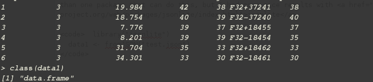
In order to be able to process these data, I had to transform it into a structured format, preferentially non proprietary, so I chosen CSV (3 stars). This was achieved using a combination of command-line processing tools (e.g.: pdftotext, sed and grep).

The next step was to publish these data, following the FAIR principles, so that it is Findable, Accessible, Interoperable and Reusable. In order to do that, I have chosen the OGC API Features standard, which allows to publish vector geospatial data on the web. This standard defines a RESTfull API with JSON encodings, which fits the expectations of modern web applications. I used a Python implementation of OGC API Features, called pygeoapi.

Before getting the data into pygeoapi, I had to georeference it. In order to do forward geocoding, I used the OpenCage API, and more specifically a Python client, which is one of the many supported SDKs. After tweaking the parameters, the results were quite good, and I was even able to georeference some incomplete addresses, something that was not possible using the Nominatum OSM API.

The next thing was to get the data into a format which supports geometry. The CSV was transformed into a GeoJSON using GDAL/ogr2ogr. I could have published it as a GeoJSON int pygeoapi, but indexing into a database adds support to more functionality, so I decided to store it in a MongoDB NoSQL data store. Everything was virtualized into docker containers, and orchestrated using this docker-compose file.

The application was deployed in AWS and the collection is available at this endpoint:

https://features.byteroad.net/collections/gas_stations

This means that anyone is able to consume this data and create their own maps, whether they are using QGIS, ArcGIS, JavaScript, Python, etc. All they need is an application which implements the OGC API Features standard.

I also created a map, using React.js and the Leaflet library. Although Leaflet does not support OGC API Features natively, I was able to fetch the data as GeoJSON, by following this approach.

The resulting application is available here:

https://ivaucher.byteroad.net

Now you can navigate through the map until you find you area of interest, or even type an address in the search box, to let the map fly to that location.

Hopefully, this application will make the user experience of the IVAucher program a bit easier, but it will also demonstrate the importance of using standards in order to leverage the use of geospatial information. Making data available on the web is good, but it is time that we move a step forward and question “how” we are making the data available, in order to ensure that its full potential is unlocked.

Data Analytics Bootcamp

I have always dreamed about doing some contribution towards improving the gender balance in technology, which as you may know, is far from ideal.

Fortunately the opportunity arose, when Katrina Walker has invited me to teach the “Data Analytics”  bootcamp at CodeOp, an international code school for women and TGNC individuals.

Over the 6-month course, I will share my hands-on experience with the various stages of the data analysis pipeline, specifically on how to apply various technologies to ingest, model and visualize data insights.

Rather than focusing on a specific technology, I will leverage on the “best tool for the job, approach”, which is what I do when I want to analyse data. This means learning different tools, such as Python, R, SQL or QGIS, and often combine them together.

For me “data analytics” is like a journey, where we start with a high-level problem, translate it into data and algorithms, and finally extract a high-level idea. At the start and the end of journey, we should always be able to communicate with people that are not “data geeks” and this is one idea that I would like to pass in the course.

I will not add anything else, apart that I am really excited to get started!

Spatial Data Mining

Social media streams may generate massive clouds of geolocated points, but how can we extract useful information from these, sometimes huge, datasets? I think machine learning and GIS can be helpful here.

My PechaKucha talk at DataBeers : “Visualizing Geolocated Tweets: a Spatial Data Mining Approach”.

Cluster Explorer Demo

Cluster explorer is a piece of software I was working on, which blends machine learning and GIS to produce a cluster visualization on top of a virtual globe.
The virtual globe uses NasaWorldWind, a Java framework for 3D geo-visualization based on OpenGL, while the clustering algorithms use the ELKI Data mining framework for unsupervised learning.
The tool allows to cluster a bunch of points (for instance geolocated Tweets) using one of two algorithms (or both), and explore the contextual information provided by the geographic layers (e.g.: OSM, Bing).

Visualizing Micro-blogging Data

This time I’m at the Workshop: “Data Visualization from Different Universes”, presenting some work regarding the visualization of Tweets, using a combination of machine learning and GIS.

Driving Spatial Analysis Beyond the Limits of Traditional Storage

My presentation on the “Conference on Advanced Spatial Modelling and Analysis” consisted in some thoughts regarding Big Spatial Data, and how to handle them in terms of modern technologies.

It was great to see such a motivated crowd from all generations, and to get to know the research developed by CEG, in topics such as Agent Based Modelling and Neural Networks. It was also great to talk again to Arnaud Banos, from the Complex System Institute of Paris Ile-de-France (ISC-PIF).

CSV 2 GeoJSON

Recently I had another challenge, which I believe has the characteristics to be a common problem. I have a table with attributes, in CSV format, one of which is geospatial.

CSV is a structured format for storing tabular data (text and numbers), where each row corresponds to a record, and each field is separated by a known character(generally a comma). It is probably one of the most common formats to distribute that, probably because it is a standard output from relational databases.

Since people hand me data often in this format, and for a number of reasons it is more convenient for me to to use JSON data, I thought it would be handy to have a method to translating CSV into JSON, and this was the first milestone of this challenge.

The second milestone of this challenge, is that there is some geospatial information within this data, serialized in a non standard format, and I would like to convert it into a standard JSON format for spatial data; e.g.: GeoJSON. So the second milestone has actually two parts:

• parse a GeoJSON geometry from the CSV fields
• pack the geometry and the properties into GeoJSON field

To convert CSV (or XML) to JSON, I found this really nice website. It lets you upload a file, and save the results into another file,so I could transform this:

TMC,ROADNUMBER,DIR,PROV,CCAA,StartLatitude,StartLongitude,
EndLatitude,EndLongitude
E17+02412,A-2,E-90/AP-2/BARCELONA-ZARAGOZA (SOSES),LLEIDA,
CATALUNYA,41.5368273,0.4387071,
41.5388396,0.4638462

into this:

{
"TMC": "E17+02412",
"ROADNUMBER": "A-2",
"DIR": "E-90/AP-2/BARCELONA-ZARAGOZA (SOSES)",
"PROV": "LLEIDA",
"CCAA": "CATALUNYA",
"StartLatitude": "41.5368273",
"StartLongitude": "0.4387071",
"EndLatitude": "41.5388396",
"EndLongitude": "0.4638462"
}

This gave me a nicely formatted JSON output (the first milestone!), but as you can notice the geometry is not conform with any OGC standards. It is actually a linestring, which is defined by a start point (StartLongitude, StartLatitude) and an end point (EndLongitude, EndLatitude).

According to the JSON spec, a linestring is defined by an array of coordinates:

So the goal would be to transform the geometry above into:

"LineString",
"coordinates": [
[0.4387071, 41.5368273], [0.4638462, 41.5388396]
]

Once more, jq comes really handy to this task.

The JSON can be transformed into a feature using this syntax:

cat tramos.json | jq -c '[.[] | { type: "Feature", "geometry": {"type": "LineString","coordinates": [ [.StartLongitude, .StartLatitude| tonumber], [ .EndLongitude, .EndLatitude | tonumber] ] }, properties: {tmc: .TMC, roadnumber: .ROADNUMBER, dir: .DIR, prov: .PROV, ccaa: .CCAA}}]' > tramos.geojson

Since the JSON converser parse all the variables into strings, it is important to pass a filter (tonumber) to make sure that the coordinate numbers are converted back into numbers.

{
"properties": {
"ccaa": "CATALUNYA",
"prov": "LLEIDA",
"dir": "N-IIA/SOSES/TORRES DE SEGRE/ALCARRàS",
"roadnumber": "A-2",
"tmc": "E17+02413"
},
"geometry": {
"coordinates": [
[
0.4714937,
41.5420936
],
[
0.4891472,
41.5497014
]
],
"type": "LineString"
},
"type": "Feature"
}

Since we are creating an array of features (or “Feature Collection”), to be conform with GeoJSON, it is important to declare the root element too, by adding this outer element:

{ "type": "FeatureCollection","features": [ ]}

The result should be a valid GeoJSON, that you can view and manipulate in your favourite GIS (for instance QGIS!) 🙂

Piping an API into R: a Data Science Workflow

Inspired by @jeroenhjanssens, author of the Data Science Toolbox, I decided to give a go to one of the most unfriendly data sources: An XML API.
Apart from its rich syntax with query capabilities, I tend think XML is highly verbose and human unfriendly, which is quite a discouraging if you don’t want to take advantage of all its capabilities. And in my case I didn’t: I just wanted to grab a data stream, in order to be able to build some analysis in R. APIs are generally a pain for data scientists, because they tend to want to have “a look at things” and get a general feeling of the dataset, before start building code. Normally, this is not possible with an API, unless you use these high-end drag-and-drop interfaces, that are generally costly. But following this approach I was able to setup a chain of tools that enable me to reproduce this AGILE workflow, where you can have a feel of the dataset in R, without having to write a Python client.

The first step was to pipe the xml output of the query into a file, and that is easy enough to do with curl

curl -s 'http://someurl.com/Data/Entity.ashx?Action=GetStuff&Par=59&Resolution=250&&token=OxWDsixG6n5sometoken' > out.xml

Now, if you are an XML wiz you can follow a different approach, but I personally feel more comfortable with JSON, so the next step for me was to convert the XML dump into some nice JSON, and fortunately there is another free tool for that too: xml2json

xml2json < out.xml > out.json

Having the JSON, it is possible to query it using jq, a command line JSON parser that I find really intuitive. With this command, I am able to narrow the dataset to the fields I am interested, and pipe the results into another text file. In this case I am skipping all the “headers”, and grabbing an array of elements, which is what I want to analyse.

cat out.json | jq '[.Root.ResultSet.Entity[] | {color: .color, width: .with, average: .average, reference: .reference, Time: .Time}]' > test.json


Now here I could add another step, to convert the JSON results into csv, but actually R has interfaces to JSON, so why not use those to import the data directly. There is actually more than one package that can do this, but I had some nice results with jsonlite.

library("jsonlite")
data1 <- fromJSON("test.json")

And with these two lines of code, I have a data frame that I can use for running ML algorithms.

Post-processing OPTICSxi Clustering

On a previous post, I expressed my concerns regarding the results of OPTICSxi clustering. Namely, I mentioned an “annoying” spike effect, that turns out massively almost at any simulation (so massively that it is almost a “feature”).

A post in StackOverflow, originated an useful exchange of ideas with the author of the ELKI framework. Namely he pointed out a “weakness” of the algorithm, that basis its partition on the reachability distance, which is not always a synonymous of “spatial closeness”. Literally, outliers that are standing in the middle of clusters, could be erroneous misinterpretated as belonging to a cluster or the other.

Since this is a problem on the partition algorithm, the solution could pass through improving the partition algorithm, using a different partition algorithm, or using a different cluster algorithm all together.  As a “quick fix” I opted to some cluster “post-processing”, in order to remove the outliers.

So my research question was: how to identify a point that is a spatial outlier?

I tried a couple of approaches that I will discuss now, as I think they may be useful for someone or generate an useful discussion.

On the image above, the coloured points are outliers, according to our definition. One simple approach, would be to calculate the average path length, the average distance of one point, to all other points in the point cloud. Then we could test the distance of each point, and say if it is greater than a certain value, let us say 5,  we would consider it an outlier and remove it from the dataset. I found this approach actually yield good results, and was able to reduce the “spikes” that we see in this figure:

To this results:

The code that calculates the average distance for each point, is bellow:

public static double getAverageDistance(Coordinate coord, ModifiableDBIDs ids, HashMap dataMap){

double sum=0.0;

try{
for (DBIDIter iter = ids.iter();
iter.valid(); iter.advance())
sum+=coord.distance(dataMap.get(DBIDUtil.toString(iter)));
}
catch( Exception  exp) {
System.out.println( "Unexpected exception:" + exp.getMessage() );
}
return sum/ids.size();
}


From the point of view of “correctness” this algorithm suffers of the “bottleneck” of removing the outlier from the clusters (and thus converting it into “noise”). To avoid this, it would have to be tested if the point actually belongs to another cluster.

Apart from that, in terms of computation the algorithm is extremely “costly” , being the most costly part when it computes the distances from all points to all points, literally a matrix of NxN that can easily increase to huge numbers with a large cluster.

To avoid that, I tried a few different approaches. One was to calculate this distances for a part of the dataset. We know that by the way the algorithm is written, the outliers tend to “appear” either in the beginning or the end of the cluster. Having this in mind, I calculated the average based on the 60% “middle” values (n<20% and n>20%) and tested the condition for the first 20% and last 20% (this refinement was actually not needed as the “costly” part of the algorithm is the distance matrix and not the condition testing). I was not able to reach any reasonable results with this approach, either because the points were not ordered (which defeats the all purpose of my “slicing”) or because outliers were appearing outside these “classes” (i.e.: in the middle of the dataset).

The other approach that I tried was to work with the “final” polygon (the convex hull of the cluster), rather than the raw points. The polygon border has only a few points, when compared to the point cloud used to generate it. It is very easy and quick to identify the “outlier” in the polygon border; however removing it, will understandable result in a “strange polygon”, since the reality is: if that point would not be used to build the polygon, another point (that we don’t have right now!) would be used, and so the real geometry would not be this one. This is particularly noticeable when we see overlapping clusters (which don’t overlap anymore). After this experience, it became clear that the processing would have to be done in the cluster point dataset, before building the polygon.

I ended up with an algorithm that successfully removes the “spike” effects from OPTICSxi, but is rather costly in terms of time (more costly than OPTICSxi itself) and unfortunately this grows exponentially with the size of the dataset, which limits its application with big data.

UPDATE

The approach above was improved, by testing the distances against the 2 neighbours of each point (previous and next point) rather than against the entire matrix. With this hack, the running time of the algorithm was reduced to reasonable values, that don’t grow up so much with the size of the vector.

Parametrizing and interpreting OPTICSxi Clustering

For a while now, I have been working on the application of the OPTICS clustering, for user generated data in cities.
OPTICS is a density-based algorithm that attempts to overcome some of the “weaknesses” of its most famous counterpart: DBSCAN. The major weaknesses of DBSCAN are:

• the inability to detect clusters in zones of varying density.
• the choice of parameter values, for which it is very sensitive.

I am using an implementation from the ELKI Data Mining libraries, which is one of the few existing ones. Unlike DBSCAN, the OPTICS algorithm does not produce a strict cluster partition, but an augmented ordering of the database. To produce the cluster partition, I use OPTICSxi, which is another algorithm that produces a classification based on the output of OPTICS. There are even fewer libraries capable of extracting a cluster partition from the output of OPTICS, and ELKI’s OPTICSxi implementation is one of the few ones.

In a nutshell, the parameters needed for the OPTICS algorithm are:

• epsilon: this parameter is meant as a “maximum” distance to consider, and not a specific distance to consider (DBSCAN); a whole range of distances is considered in the OPTICS algorithm, up to epsilon; although we can choose an “extremely” large epsilon, that will increase the time the algorithm will take to converge;
• minpts: this is the number of points required to form a cluster (the same as in DBSCAN);

The OPTICSxi algorithm adds an “extra” parameter:

• xi: contrast parameter, that establishes the relative decrease in density; this parameter controls directly the number of classes we will obtain.

Taking in consideration what I wrote above, if we “replace” DBSCAN by OPTICxi, we will still have to choose a min points, the epsilon will become less important (but we still need to set it), and suddenly we have a “new” parameter to set: xi. I am not completely sure this is a gain in terms of easier parametrization….

It is very clear to me, how-to interpret the results of DBSCAN (although it is not that easy, to set “meaningful” global parameters); DBSCAN detects a “prototype” of a cluster, characterized by a density, expressed as a number of points per area (minpts/epsilon). The results of OPTICSxi seem a bit more difficult to interpret.

The clusters generated by OPTICSxi are hierarchical, where “outer” clusters (lower in the hierarchical scale), contain inner clusters (or “child” clusters). Looking at the algorithm, it is clear that the idea of varying densities, is implemented by having a range of epsilon parameters, that is actually based on the data. When we set the “contrast” parameter, we actually “decide”, which density variation we accept, in order to consider that group a cluster. Because the algorithm is focused on “density variation”, rather than on a global value of density (or a “prototype”), it may well happen that areas that have a very low density appear as a cluster, just because they have a density variation from their surrounds that is greater than the accepted threshold. Likewise, we may have areas that are extremely dense, and are not detected as clusters, because there is a smooth density variation from their surroundings. In terms of interpretation this may well result in a bottleneck.

On the image bellow, we see clusters in parts of the city that are not particularly dense (like the West) and are not detected as clusters by DBSCAN. On the other hand, the centre of the city (more dense), as only a few clusters.

epsilon=500; xi=0.03; minpts=150;

It is interesting to note, that since OPTICS does not impose a strict “prototype” of density, the clusters in denser areas (in the centre of the city) are smaller in area than the clusters in less dense areas (the surroundings).

There are two phenomena that I sometimes detect in the outputs of OPTICSxi, and that I am not able to explain. One is the appearance of “spike” clusters, that link parts of the map. I cannot explain them, because they seem to be made of very few points and I don’t understand how the algorithm decides to group them in the same cluster. Do they really represent a “corridor” of density variation? looking at the underlying data, it does not look like that. You can see these “spikes” in the image bellow.

epsilon=1000; xi=0.05; minpts=100;

The other phenomenon that I cannot explain is the fact that sometimes there are overlapping clusters of the same hierarchical level. OPTICSxi is based on the OPTICS ordering of the database (e.g. dendrogram) and there are no repeated points in that diagram.

http://en.wikipedia.org/wiki/OPTICS_algorithm

Since this is a hierarchical clustering, we consider that clusters of a lower level contain clusters of a higher level, and that idea is enforced when building the convex hulls. However, I don’t see any justification for having clusters that intersect other clusters on the same hierarchical level, which in practice would mean that some points would have a double cluster “membership”. On the image bellow, we can see some intersecting clusters with the same hierarchical level (0).

Finally the most important thought/question that I want to leave you with, is: what do we expect to see in an OPTICSxi cluster classification? This question is closely linked to the task of parametrizing OPTICSxi.
Since I see hardly any studies with runs of OPTICSxi for a particular cluster problem, I struggle to find what is an optimal clustering classification would be; i.e.: one that can provide some meaningful/useful results, and add some value to the DBSCAN clustering. To help me answering that question, I performed many runs of OPTICSxi, with different combinations of parameters, and I selected three that I will discuss bellow.

epsilon=2000; xi=0.025; minpts=100;

On this run I used a large value of epsilon (2Km); the meaning of that value is that we accept large clusters (up to 2Km); since the algorithm “merges” clusters, we will end up with some very large clusters, that will have almost certainly a low density. I like this output, because it exposes the hierarchical structure of the classification, and it actually reminds me of several runs DBSCAN with a different combination of parameters (for different densities), which is the advertised “strength” of OPTICS. As it was mentioned before, smaller clusters correspond to higher levels in the hierarchical scale, and higher densities.

epsilon=250; xi=0.035; minpts=10;

On this run we see a large number of clusters, even if the “contrast” parameter is the same from the previous run. That is mostly because I chosen a low number of minpts, which established that we accept clusters with a low number of points. Since the epsilon in this case is shorter, we don’t see these large clusters occupying a large part of the map. I find this output less interesting than the previous one, mostly because, even if we have an hierarchical structure there are many clusters at the same level, and many of them intersect. In terms of interpretation, I can see an overall “shape” that is similar to the previous one, but it is actually discretized in lots of small clusters that are easily overlooked as “noise”.

epsilon=250; xi=0.035; minpts=100;

This run has a parameter choice that is similar to the previous one, except that the minpts is larger; the consequences is that not only we find less clusters and they overlap less, but also that they are mostly at the same level.

In a perspective of adding value to DBSCAN, I would opt for the first combination of parameters, since it provides a hierarchical picture of the data, exposing clearly which areas are more dense. IMHO the last combination of parameters, fails to provide an idea of the global distribution of density, since it is finding similar clusters all over the study area.